You have taken time to create a product sales PivotTable and now you would like to analyze the data. You want to analyze the sales per branch by quickly generating PivotTables for each branch to be placed on separate worksheets.
In this week’s tip, we take you through a few easy steps as we show you how this process can be easily automated.
Note: You are welcome to download the workbook to practice.
Applies To: Microsoft® Excel® 2007,2010,2013,2016.
1. Open the practice workbook and select any cell within the data list.
2. Select Insert–PivotTable and then select OK.
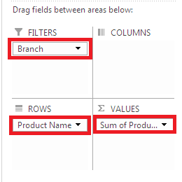
3. An empty PivotTable will open on a new worksheet. Refer to the PivotTable field list and place the fields as follows.
a. Branch: Filters Area.
b. Product Name: Rows Area.
c. Product Sales: Values Area.

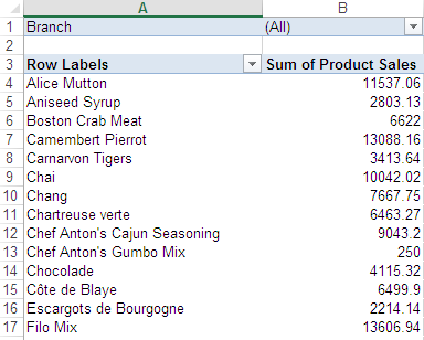
4. Your PivotTable will now appear as follows:
 Note: Branch in the Filters Area.
5. You now want to display the Branch details on individual worksheets:
a. Go to the Analyze Tab, select the drop down arrow next to Options, and select Show Report Filter Pages and select OK.

6. The individual details will be displayed on separate worksheets.
Your sales data for the different branches will be extracted and placed on separate worksheets, thus making it easier to view and analyze your sales data at a glance, which allows for better decision making.

