This week’s tip is especially handy when running competitions for your business, so please share it with your promotions and marketing teams. The Sampling Analysis Tool is great for when you need to randomly select a number from a given range of values. An example of this is the following; say your marketing team is running a lucky draw competition and needs your help in selecting a winner by random, you can use the Sampling Analysis tool to ensure that this winner is selected without favour.
This tool selects a random sample from your range of values (a sample being a portion of the whole range), therefore ensuring that your competition winner has been chosen with integrity.
Note: You are welcome to download the sample workbook to practice this exercise.
Applies to: Microsoft Excel 2007, 2010 and 2013
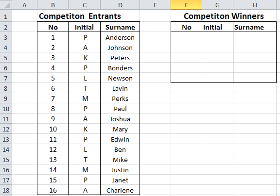
The screen shot below will be used for this example.

1. Select the Data tab and Data Analysis as per screen shot below.

N.B: If the Data Analysis option is not installed, you can install it by following the instructions below:
- Select the Microsoft Office button or the File tab, and then select Excel Options/ Options.
- Select Add-Ins, and then in the Manage box drop-down list, select Excel Add-ins, then select Go.
- In the Add-ins available box, check the Analysis ToolPak box, and then select OK.
- If Analysis ToolPak is not listed in the Add-ins available drop-down list, select Browse to locate it.
- If you get prompted that the Analysis ToolPak is not currently installed on your computer, select Yes to install it.
- After you load the Analysis ToolPak, the Data Analysis command is available in the Analysis group on the Data tab.
2. Select the Data Analysis command as per the screen shot below.
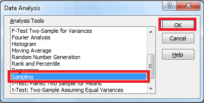
3. Select Sampling and then OK.

4. Then select or type in the Input Range, Number of Samples and Output Range as below. Select OK.

5. The results will be displayed as reflected in the image below.

6. Use Vlookup to extract the initials and surnames of the competition winners.
7. Select cell G3 and enter the following Vlookup formula: =VLOOKUP(F3,$B$2:$D$18,2,0)
8. Press Enter and copy the formula down to cell G7.
9. Select cell H3 and enter the following Vlookup formula: =VLOOKUP(F3,$B$2:$D$18,3,0)
10. Press Enter and copy the formula down to cell H7.
11. The initials and surnames will be displayed as below.

Not only will the Sampling Analysis tool make choosing your winner fair, but also help make your process more efficient and effective, saving you time and money.

